Flux and Fields

We used this apparatus to determine how angle  decreasing would effect the overall flux in an electric field ( the number of nails)

We used Loggerpro to determine the graphical behavior of the flux

We observed a sinusoidal behavior where the flux or nail decreased

We determined that the flux was dependent on the net charge enclosed in the Gaussian surface

Throughout this lab we wanted to observe and calculate the behaviors of flux in certain situations

The Electric Field

We used ActivPhysics to answer the above questions that pertained to the behavior of particles of like charge, opposite charge, or differing magnitudes. We varying the distances, number of particles, and charges to observe their behavior with each other

We were given an extended charge distribution. We were given an insulated object with uniformly distributed charge and were excepted to compute the corresponding electric field experienced by a given point at a given distance d. We utilized excel to do most of the calculations to give an approximate value as to what the point p would be experiencing if it was a charged particle.

We were given the assignment to use an interactive program to demonstrate the behaviors a charged particle or in the case of the game the "puck"  would experience as a result of the attributes that another charged particles would exert on it due to its electrical field.

Throughout this lab we discussed and conducted experiments to demonstrate the behavior particles go through when in the presence of another particle , where they would experience a force and therefore an electric field. We observed the superposition principle where multiple charges were in the same given area of each other.

Electric Static Force

 
 

We observed the tape would repel when both pieces of tape had the same charge and attract when they had been oppositely charged.

Here we used a force diagram to solve and determine the force inflicted by the charged ball as it approached a ball of same charge but connected to a string and thus created an angle we used to solve for the electric force it was experiencing.

 We applied the tape designated with a top and bottom portion onto the table. We expected charge to either be induced or transferred since it was in contact with the surface of the table.

Here after graphing our data and fitting our graph we observed a 1 / r^2 relationship between the particles and their electric force, where the closer the particles were the larger the force became as evident by the graph.

The definition of the electric force showed that 1/r^2 we in our experimental data found it to be 1.8 so we ended up with a 19.0 percent error between the experimental value and the actual value. since we manually recorded the points in the video that tracked the moti0n of the particle we expected to have some error in our tracking consistency.

Throughout this lab we sought to establish characteristics and relationships that govern the behavior of charged particles that were either static or moving very slowly. We began by conducting qualitative experiment's to demonstrate how real objects behave under conditions of electro static  influence. We showed that a charged balloon induced an attraction between it and a glass surface. Next, we showed the repelling force between two like charges in the tape experiment. Finally, we used our knowledge gained with the two previous experiments to find a quantitative equation for the electric force we had been observing. We observed two like charges, one attached to static point and the other moving toward the other ball, which caused an angular displacement, we used that angular displacement with the aid of force diagrams and math to come up with an equation that modeled the force that the charges were producing.

Heat Engines, Refridgeration, and Entropy

We were given a diesel cycle PV graph, which we were to use to determine pressure, volume, and temperature at given points as well as the heat, work, internal energy, and entropy at sections between points. As a result, we should be able to calculate the efficiency of the engine given the information provided and  necessary equations.

At different point's and steps we used the various equations that were needed for adiabatic compression, constant pressure, and constant volume. Furthermore, we used our understanding of the relationships under certain conditions to eliminate either Q, W, or delta U.

We were supposed to get a total internal energy of zero based on the theory of a cycle, which states that between the work and heat transfer the overall system should be zero at the end. I ended up getting 50 J over which I failed to find the mistake.

Heat Engines and Thermodynamics

The P-V cycle is used here to find the different states and how to use those states to find the energy. We used the first law of thermodynamics to eliminate either W depending on the conditions of constant velocity. We also used the idea of delta E= nRT3/2 to find the  change of energy between to points.

The Carnot engine cycle is what we used here it alternated between states of adiabatic and isobaric. We used these ideas to understand that at certain points the heat transfer Q is zero, also under constant pressure delta V is proportional to the temperature. If Q was zero between points we used delta E = W for the change in volume was it did work.

Here we had a isochoric situation where the temperature increase was proportional to the deltaE increase, since work was zero

Here we had a situation of isobaric where the work increased with a volume change and the higher  heat change increased created a somewhat linear increase in delta E.

Here we solved for the specific heat under conditions of constant pressure

State Variables and Ideal Gas laws

The Fire Syringe we used to find the final temperature in an insulated system where we quickly heated the system to create minimal heat transfer from cylinder striking the material out of the tube.



Here on the bottom we did work on the system in insulated conditions, compressing the volume of air inside the cylinder and raising the internal heat causing a combustion.

hb

We use the dimensions of the cylinder to calculate volume using the relationship pi r^2 L ,where we had an L initial and L final, and a given radius, we used room temperature at 24 degrees Celsius then converted  to kelvins

Charles law I

 

 

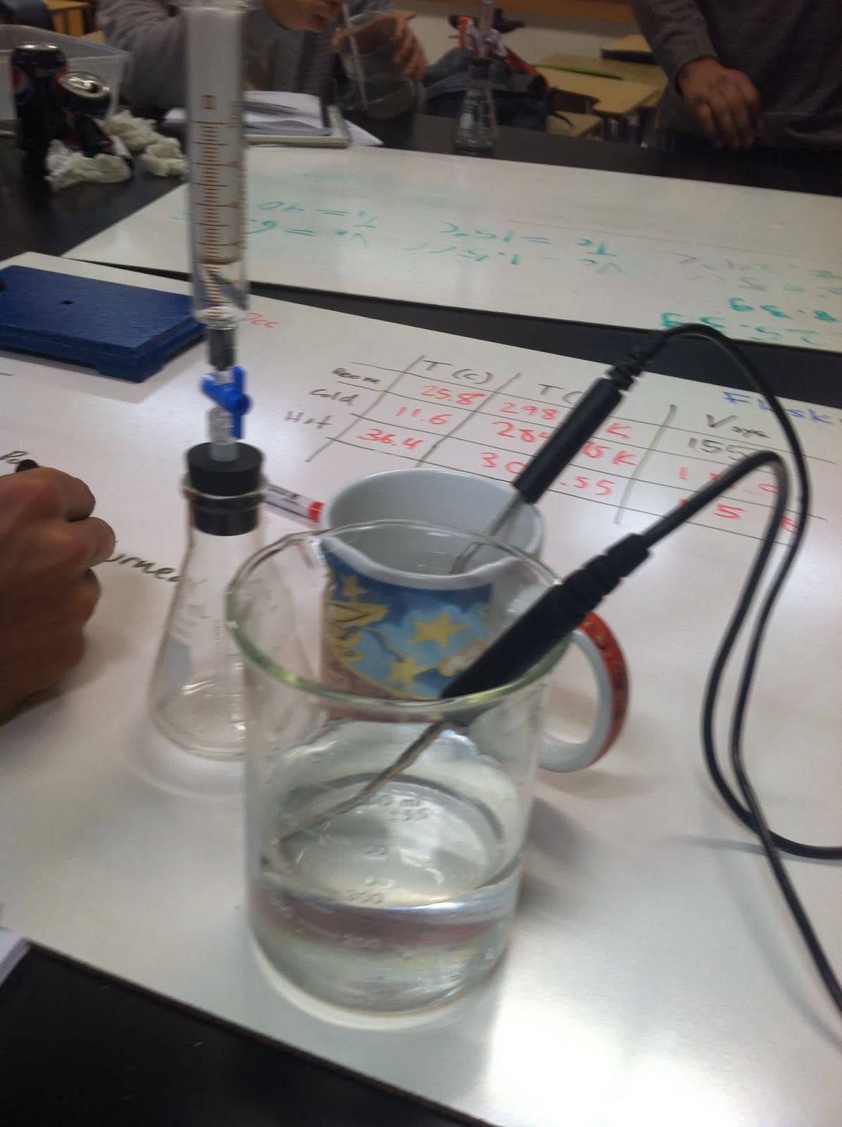
We utilized these devices to try and identify a relationship between temperature change and volume change.

 

 

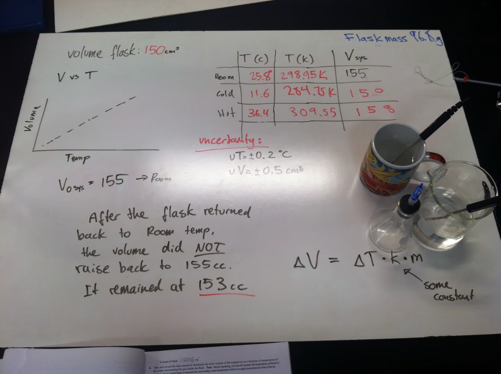
We observed in our experiment with pressure being constant, as the temperature increased, so did the volume, likewise as the temperature decreased, so did the volume, thus giving evidence of a proportionality between the two measurements. V/T=nR/P with right side being constant

 

We graphed our data to confirm what we believed to be a proportionality between Temperature and volume at constant pressure. The slope V/T  had units cm^3/ K and constant of 1/3, which displayed what we observed I our data table.

 

We did the experiments to observe the relationships and behaviors of various variables T,V, P under certain conditions. Observing the experiments, solving the equations, and plotting the graphs served to fully understand the important aspects of the gas laws specially ideal.